How To Filter On Google Sheets - If you’re wondering how this works, go through a couple of examples (listed below) and it will become clear on how to use the filter function in google she.

July 18, 2021

How To Filter On Google Sheets - If you're wondering how this works, go through a couple of examples (listed below) and it will become clear on how to use the filter function in google she.. The profit for flour in utah was 1240, and the filter function ignored it because it did not meet the second condition. Now you can see a dropdown arrow appear on the header row of every column. This is an optional argument and can be the second condition for which you check in the formula. Click the filter icon in the header for the column that you want to filter. Similarly, if you want, you can have multiple conditions in the same filter formula.

The below formula will do this: How do you filter columns in google sheets? Reset the filters applied in the previous step (simply click on the funnel icon again to turn off the filter). Or click on the filter button on the toolbar. This would return all the records that match the criteria, which would be the top three records.

Filter By Condition In Google Sheets And Work With Filters In Shared Documents from cdn.ablebits.com

Below is the formula that will filter all the even rows: The above formula uses the addition operator in the condition to first check both the conditions and then add the result of each. The above formula uses the row function to get the row numbers of all the rows in the dataset. This will give you 0 (or false) where both the conditions are not met, 1 where one of the two conditions are met, and 2 where both the conditions are met. Google sheets also tells you why it. The above formula takes the data range as the argument and the condition is b2:b11="florida". For example, suppose you have the dataset as shown below and you want to get all the records for california and iowa. See full list on spreadsheetpoint.com

This will give you 0 (or false) where both the conditions are not met, 1 where one of the two conditions are met, and 2 where both the conditions are met.

For example, if you have the text florida in cell h1, you can also use the below formula: Jun 28, 2021 · if you use color in your spreadsheet to highlight text or cells, you can filter by the colors that you use. This would return all the records that match the criteria, which would be the top three records. See full list on spreadsheetpoint.com May 24, 2021 · 2. Click on the create a filter option. Jan 08, 2020 · here's how to create one: The above formula checks for two conditions (where the state is florida and sale value is more than 5000) and returns all the records that meet these criteria. You can also use the filter function to check for multiple conditions in such a way that it only returns those records where both the conditions are met. For example, suppose i have the dataset as shown below and i want to quickly get the records for the top 3 sales values. The profit for flour in utah was 1240, and the filter function ignored it because it did not meet the second condition. This needs to be of the same size as that of the range. You can do this using the below formula;

How do i sort table in google sheets? Press enter to execute the formula. A few things to know about the filter function. You can also use the filter function to check for multiple conditions in such a way that it only returns those records where both the conditions are met. For example, suppose i have the dataset as shown below and i want to quickly get the records for the top 3 sales values.

Spreadsheet Tips Filters In Google Sheets Filter Views Individualised Filters Youtube from i.ytimg.com

In case you want to get the bottom three records, you can use the below filter formula: This condition checks each cell in the range b2:b11 and if the value is equal to florida, that record is filtered, else it's not. Click the filter icon in the header for the column that you want to filter. The below formula will do this: In case you leave it blank (or make it true), the result will be in ascendin. If you're wondering how this works, go through a couple of examples (listed below) and it will become clear on how to use the filter function in google she. See full list on spreadsheetpoint.com May 24, 2021 · 2.

Jun 02, 2021 · selecting the right dataset to apply filter to keep the gap between columns in place, manually select the whole dataset.

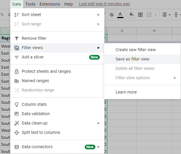
If any of the cell(s) is not empty, your formula will return a #ref! Many times, the data you need will only be in alternate rows (or every third/fourth/fifth row), and you would have a need to get rid of the extra rows so that you can get all the useful data together. Press enter to execute the formula. The below formula will do this: This condition checks each cell in the range b2:b11 and if the value is equal to florida, that record is filtered, else it's not. The above formula uses the addition operator in the condition to first check both the conditions and then add the result of each. The below formula will do this: Select data filter views create new filter view. See full list on spreadsheetpoint.com May 24, 2021 · 2. In case you leave it blank (or make it true), the result will be in ascendin. This value is then used in the condition to check whether the values in column c are greater than or equal to this value or not. In order to use an or condition, all you need to do is put the conditions in brackets and add them together with a plus sign, instead of separating them by a comma.

It then subtracts 1 from it as our dataset starts from the second row onwards. In case you want to get the bottom three records, you can use the below filter formula: See full list on spreadsheetpoint.com And then the filter formula will return all the records where the conditions return value more than 0. This is the columns/row (corresponding to the column/row of the dataset), that returns an array of trues/falses.

How To Filter Rows Based On Cell Color In Google Sheet from cdn.extendoffice.com

This is the range of cells that you want to filter. Suppose you have the dataset as shown below and you want to quickly filter all the records where the state name is florida. For this to work, you need to make sure that the adjacent cells (where the results would be placed) should be empty. Below is the formula that will filter all the even rows: The above formula uses the large function to get the third largest value in the dataset. How can i remove all filters in a google spreadsheet? In case you want to get the bottom three records, you can use the below filter formula: A few things to know about the filter function.

See full list on spreadsheetpoint.com

This means that the condition should be the state is either california or iowa (which makes this an or condition). Choose the profit column as a range for the second condition, and the new formula looks like this: The third argument in the sort functionis false, which is to specify that i want the final result in descending order. Below is the formula that will filter the data and show it in descending order: Since these conditions return an array or trues and falses, you can add these (since a true is 1 and false is 0 in google sheets). In case the filter function can not find any result that matches the condition, it would return an #n/a error. Similarly, if you want, you can have multiple conditions in the same filter formula. Reset the filters applied in the previous step (simply click on the funnel icon again to turn off the filter). Press enter to execute the formula. Click the filter icon in the header for the column that you want to filter. See full list on spreadsheetpoint.com Google sheets also tells you why it. You can also check for or condition in the filter formula.